Efficiency-oriented phased urban green space planning framework to mitigate heat-stress exposure

Study area and data sources

This study was conducted in the four core districts of Kunming, the capital of Yunnan Province, China: Guandu, Panlong, Wuhua, and Xishan. These districts lie between longitudes 102°21′ to 103°03′ E and latitudes 24°40′ to 25°17′ N, and collectively surround Dianchi Lake. In 2024, these districts spanned 2292 km² (10.91% of the city’s total area), 4.816 million residents (55.81% of the city’s population), and generated 518.86 billion RMB in GDP (65.97% of the city’s economy). Due to dense development and the exacerbation of the UHI effect, these districts face considerable challenges related to heat-stress exposure²². Hence, they were selected as a representative case study area for addressing UGS planning aimed at mitigating heat-stress.

To support the modeling framework, multiple datasets were integrated: (1) hourly mobile-phone signaling data from Chinese operators on October 16 and 17, 2023, resampled to a 70 m resolution to produce dynamic population distributions; (2) remote sensing derived LST datasets, ECOSTRESS LST (3–5 day revisit, 70 m) and CGLOPS LST (hourly, 5 km); (3) meteorological station observations from the China Meteorological Administration, including hourly air temperature, wind speed, humidity, and air pressure; and (4) land cover types from the China Land Cover Dataset (CLCD), including cropland, forest land, shrubland, grassland, water body, bare land, impervious surface, and wetland²³.

LST data fusion and thermal field construction

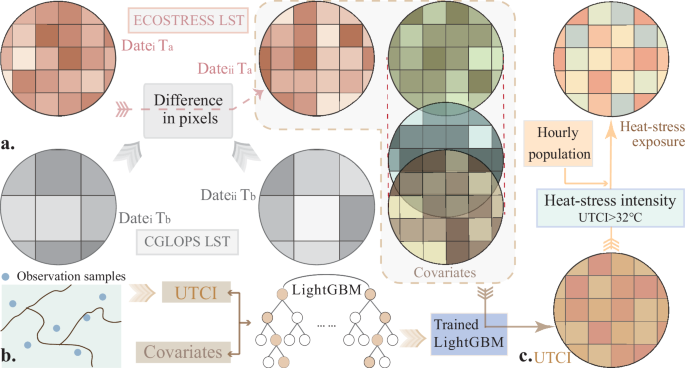
To capture hourly LST at high resolution, we fused ECOSTRESS and CGLOPS LST data through a temporal anomaly-based bias correction (Fig. 5a). For each hour of May 31, 2023 (statistically the hottest day), we adjusted ECOSTRESS LST using the deviation between CGLOPS LST on the target and observation days²⁴. This method inherits the spatial granularity of ECOSTRESS LST data and the temporal continuity of CGLOPS LST data. A sliding window algorithm was applied for temporal smoothing¹⁵, reducing edge artifacts while preserving temperature gradients and spatial textures. The resulting 70 m resolution hourly LST data served as inputs for human thermal comfort modeling.

a Acquisition of multi-period LST datasets; b conversion of LST to the UTCI; and c calculation of heat-stress exposure.

Heat-stress and exposure modeling

To estimate human-perceived heat-stress, we reconstructed hourly UTCI data using a machine learning approach (Fig. 5b). The UTCI was predicted using a Light Gradient Boosting Machine (LightGBM) model trained on 600 station-calculated UTCI samples^25,26. Model inputs included the fused LST (hourly, 70 m), Kernel Normalized Difference Vegetation Index (kNDVI), Bare-soil Index (BI), and Index-based Built-up Index (IBI)^27,28, from temporally aligned Landsat data.

We quantified heat-stress intensity applying a 32 °C threshold, which represents strong heat-stress in the UTCI classification system²⁵. For each pixel, heat-stress intensity (\({H}_{i,t}\)) was calculated using Eq. (1).

Heat-stress exposure (\({E}_{i,t}\)) was obtained by multiplying \({H}_{i,t}\) with population data \({P}_{i,t}\) using Eq. (2).

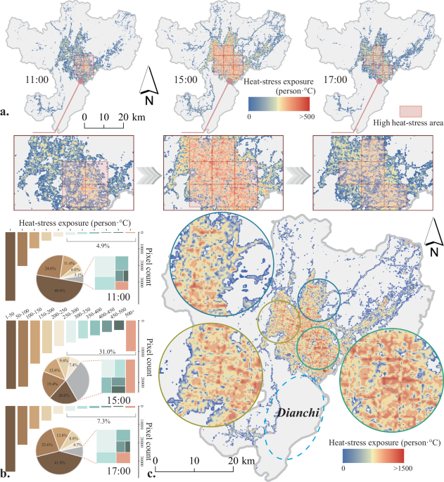
Heat-stress exposure maps were generated for the time 11:00, 15:00, and 17:00, and aggregated to reflect cumulative heat-stress exposure (Fig. 5c). Although nighttime heat-stress often exacerbates chronic health risks, especially for vulnerable groups without access to cooling, in Kunming, nighttime temperatures exhibit a significant cooling trend, with daytime peaks driving acute heat-stress exposure. Therefore, our study focused primarily on daytime periods when thermal discomfort was most pronounced.

Modeling and simulation of UGS cooling-zones

To quantify the spatial extent of UGS cooling and simulate its potential expansion under additional-UGS planning scenarios, we established a two-stage modeling framework that first extracteds measurable cooling-zones from existing-UGS and then applied a relationship model to estimate cooling-zones for additional-UGS.

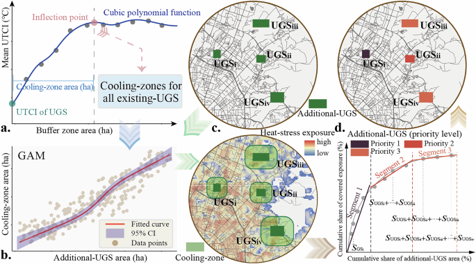
The cooling-zone of a UGS patch is defined as the spatial area where UTCI values are significantly reduced due to vegetation-induced microclimatic effects, and beyond which such influence becomes negligible. Empirical evidence supports a positive correlation between UGS size and its cooling-zone area, though this relationship is nonlinear and saturates beyond a certain size threshold²⁹. We selected the UGS from the land cover dataset, specifically forest land, shrubland, and grassland classes, and excluded patches exceeding 100 ha to avoid bias from large UGS. For each UGS, we constructed concentric buffer zones at incremental distances (scaled by 0.2 time of its own area) and extracted mean UTCI values for each buffer ring using previously reconstructed UTCI maps. The mean UTCI values were plotted against cumulative buffer area and fitted with a cubic polynomial regression (Fig. 6a).

a Cooling curves of existing-UGS and identification of cooling-zones; b relationship between UGS area and cooling-zone area; c simulation of cooling-zones for additional-UGS; and d determination of planning priorities for additional-UGS.

The first derivative of the fitted curve was computed to determine the inflection point (the distance at which the UTCI rising rate diminishes to zero) indicating the boundary of the UGS’s effective cooling influence³⁰. This threshold was used to delineate the cooling-zone. UGS lacking a clear inflection point were excluded from model calibration to ensure robustness. Once cooling-zones were extracted, we paired each with its originating UGS area to apply a Generalized Additive Model (GAM)³¹. This nonparametric regression framework captures nonlinear relationship and threshold effects between UGS area and associated cooling-zone area (Fig. 6b).

We identified additional-UGS for potential development, including two categories: Undeveloped greening sites (bare land), which can be transformed through ecological restoration; Existing-UGS with no detectable cooling effect, which may be enhanced via vegetation density improvements. For each additional-UGS, we applied the GAM-derived function to simulate its cooling-zone based on its area (Fig. 6c). Where simulated cooling-zones overlapped, corresponding additional-UGS were merged to form composite units, and the cooling-zone delineation process was repeated using combined area to reflect cumulative effects. Finally, the simulated cooling-zones were overlaid with spatially aligned heat-stress exposure maps. This enabled us to estimate, for each additional-UGS, the total heat-stress exposure it could potentially cover, thus forming the analytical basis for prioritization under the UGS planning framework.

Efficiency-oriented phased UGS planning

To facilitate efficiency-oriented UGS planning strategy, we developed a phased planning framework that assigns implementation priorities to additional-UGS based on their planning-efficiency. For each additional-UGS patch, planning-efficiency was quantified as the amount of heat-stress exposure covered per unit area of additional-UGS patch. All additional-UGS patches were ranked in descending order of planning-efficiency. To assess the distribution of mitigation benefits, we constructed a Lorenz curve³², by plotting the cumulative share of additional-UGS area (x-axis) against the cumulative share of heat-stress exposure coverage (y-axis) (Fig. 6d). This curve was used to examine the differences in heat-stress exposure coverage potential across the additional-UGS set.

To convert the continuous planning-efficiency ranking into a practical phased UGS planning strategy, we applied a data-driven classification method combining change-point detection and piecewise linear function fitting to the Lorenz curve³³. This approach identified key thresholds in the planning-efficiency distribution, which were used to segment the additional-UGS into separate planning priority levels (Fig. 6d). Each priority level represents a tier of planning urgency, with high-priority assigned to additional-UGS that demonstrate greater heat-stress exposure coverage per unit area. This classification supports phased implementation, enabling planners to allocate resources progressively, from the most efficient additional-UGS to those with more limited marginal returns.

Reporting summary

Further information on research design is available in the Nature Research Reporting Summary linked to this article.